Tolerancing and its Role in Illumination and Nonsequential Optical Design
![]()
This guest contribution on the Altair Blog is written by Dave Jacobsen, Senior Application Engineer at Lambda Research Corporation and who is a member of the Altair Partner Alliance.
Introduction
Tolerancing is a subject that is often overlooked, or not fully addressed, in the design of illumination and nonsequential optical systems. Tolerancing methods are well developed and understood in the lens design and imaging system design fields, but tolerancing of illumination and nonsequential optics is a much less well-developed field. Optical design and optimization software tools can allow the designer to make new and exciting designs, but it is possible that the design may not be economical to manufacture due to the sensitivity of the design to variations in the manufacturing process.
New tolerance analysis tools in optical design and analysis software allows designers and engineers to evaluate the effect of manufacturing variations and how it will affect the overall performance of the system. This makes it possible to see if a design is truly practical and economical. We will look at the tolerancing methodology as well as some tolerancing examples in this article.
One definition of tolerance in the Merriam-Webster online dictionary is: the allowable deviation from a standard; especially: the range of variation permitted in maintaining a specified dimension in machining a piece. In optical and illumination design this is used to define how much a manufactured design can deviate from the optimized or “perfect” design and still deliver an acceptable level of performance. An optical designer will realize that the part that is produced based on their design may not fully match the original design. A tolerant design is one that will still perform within a give range despite these inevitable differences due to manufacturing.
Many computer based optical design and analysis programs feature powerful optimization tools that optical engineers and designers can use to design complex and high performance components and systems for lighting and illumination applications. In some cases, these designs may not translate well to a production environment. Figure 1 shows an optimized luminaire reflector that would be difficult to produce accurately and consistently. Fortunately, some of these same software tools can also allow the capability to check the tolerance of a design to see if changes to the base design need to be made.
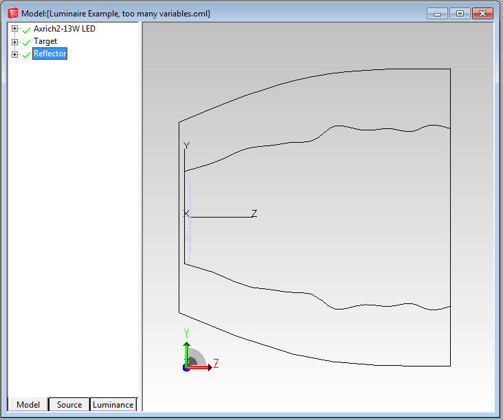
Figure 1: Reflector with complex shape
Tolerancing in Optical Systems
Tolerance analysis is lens and imaging system design is a well-established and understood field. Optical design programs such as OSLO, CodeV, and others, feature robust tolerancing routines. The initial tolerance data in OSLO for example is based on the default manufacturing tolerances outlined in the ISO 10110 drawing standard. Users are then able to change this initial tolerance data by referencing the correct class of data: Surface Tolerance Data, Component Tolerance Data, and the User-Defined-Group Tolerance Data1. The user can then select the tolerance method to use. The methods available may include, Monte Carlo analysis, Hopkins-Tiziani-Rimmer (HTR) method, user-defined tolerance, computer change table, and distributed change methods.
Tolerancing in Illumination and Nonsequential Optical Systems
Tolerance analysis in imaging/non-imaging/nonsequential designs is a much newer and less well-developed process. Some examples of non-imaging type designs are illumination and lighting, light guides and displays, and solar collectors and concentrators. The goal of the process is the same though, to perturb the initial design in a systematic way and analyze the effect of these changes on the systems performance. The performance metrics can include, flux, illuminance values, illumination pattern, uniformity, beam width, candela values, intensity pattern, luminance, and color coordinates.
When a system tolerance analysis is to be performed, the first step is to identify the parameters in the design that can change during the manufacturing process. These parameters can include curvature, aspheric terms or deviation from a spherical surface, dimensional changes, changes in conic curvatures and conic constants, misalignment of sources such as LEDs, variations in source output, changes in surface finish, and other changes in material and/or surface properties.
Once the parameters that can change have been identified and defined, the next step is to determine by how much these parameters can change. This information may come from past experience, discussions with vendors, sample measurement, and/or experimentation. In many cases it may be a combination of several sources of information. After the range of parameter variation is determined, the method for choosing values within that range during the tolerancing process can be selected. Options can include Normal or Gaussian, Uniform, or End Point analysis.
The Normal or Gaussian method will distribute the values in a Gaussian distribution centered on the nominal value with the high and low limits of the parameters as the limits for the Gaussian curve. A Uniform distribution will evenly spread the values across the range of the parameter value. An End Point analysis will test the high and low values for the parameter.
The Gaussian distribution may be a good choice when the changes are distributed around the nominal value and there is a lesser chance of the values being far from the nominal condition. The Uniform distribution is a good choice if the likely distribution of changes is not well known and the user wants to sample the entire range of possibilities with no specific weighting function. The End Point option allows for a quicker tolerance analysis by only testing the maximum deviations from nominal values.
The Gaussian or Uniform options can be used to scan through a range of values for a parameter. For example, if the radius of curvature of a surface for a TIR hybrid lens can vary by +/- 1mm. the Gaussian or Uniform options will allow the user to scan through values in the range. The End Point option can be useful to scan the maximum and minimum range of the parameter values to see the range of the performance change in the design. This can be a good option when there are numerous parameters to evaluate. After an initial analysis is used to identify the most troublesome parameters, additional analysis can also be run using more trials or a different method such as Normal/Gaussian or Uniform.
The Monte Carlo method can be used in illumination optics tolerancing. The Monte Carlo method uses random numbers to generate a sequence of optical elements, such as reflectors or lenses, determined by the upper and lower limits defined by the user. Each random iteration defines a new version of the optical element. This method allows all of the parameters to be varied or perturbed simultaneously, greatly speeding up the tolerancing process.
Setting up a Tolerance Analysis
The tolerance analysis process can be broken down into a series of steps.
1.Identify the parameters that are to be varied or changed during the tolerance analysis
2.Determine the range of motion or limits for those parameters
3.Select the method for varying the parameters
4.Choose the number of iterations to run. More iterations will generally result in more accurate representation of the results.
5.Run the tolerance analysis
6.Analyze the results and make changes/corrections if necessary
There is no limit to the number of parameters that can be varied during the tolerance analysis, though when multiple parameters are varied it may be more difficult to determine the contribution of each parameter to the variations shown in the tolerance analysis. The range of motion or limits for the parameters should be set to reflect the expected variations that would be seen in the manufacturing process or due to changes in materials or surface finishes. If the range is set too large, it can lead to a longer runtime than necessary for the tolerance analysis. As mentioned above, the variation method, typically either Gaussian or uniform, should be choose based on distribution of values that could result in the actual system.
The number of iterations to run along with the number of the rays defined in the optical analysis software will be the biggest factors in the time it takes to complete the tolerance analysis. The number of rays in the optical analysis should be chosen to give a result with enough resolution or low enough signal-to-noise ration that the results can be considered valid and meaningful. Generally, you will want to trace a large number of rays. Likewise, you will want to use enough variations to fully sample the range of expected variations in the defined parameters.
The tolerance analysis itself is an iterative process. One of the parameters will be moved, a raytrace run, and an error value is calculated. The error value is based on how well the simulated results match the user defined performance criteria, such as flux, irradiance, uniformity, beam pattern, etc.. The lower the error value the closer the simulated result is to define performance criteria. This process repeated for the number of iterations defined with the parameters being varied by a different value in each iteration.
Illumination System Tolerance Analysis Examples
Example 1: Reflector tolerance This example will show a tolerance analysis of a reflector used in a LED luminaire. The reflector has been optimized to produce and even illumination pattern in the central 25% of a target. Figure 2 shows the initial design and illumination pattern.
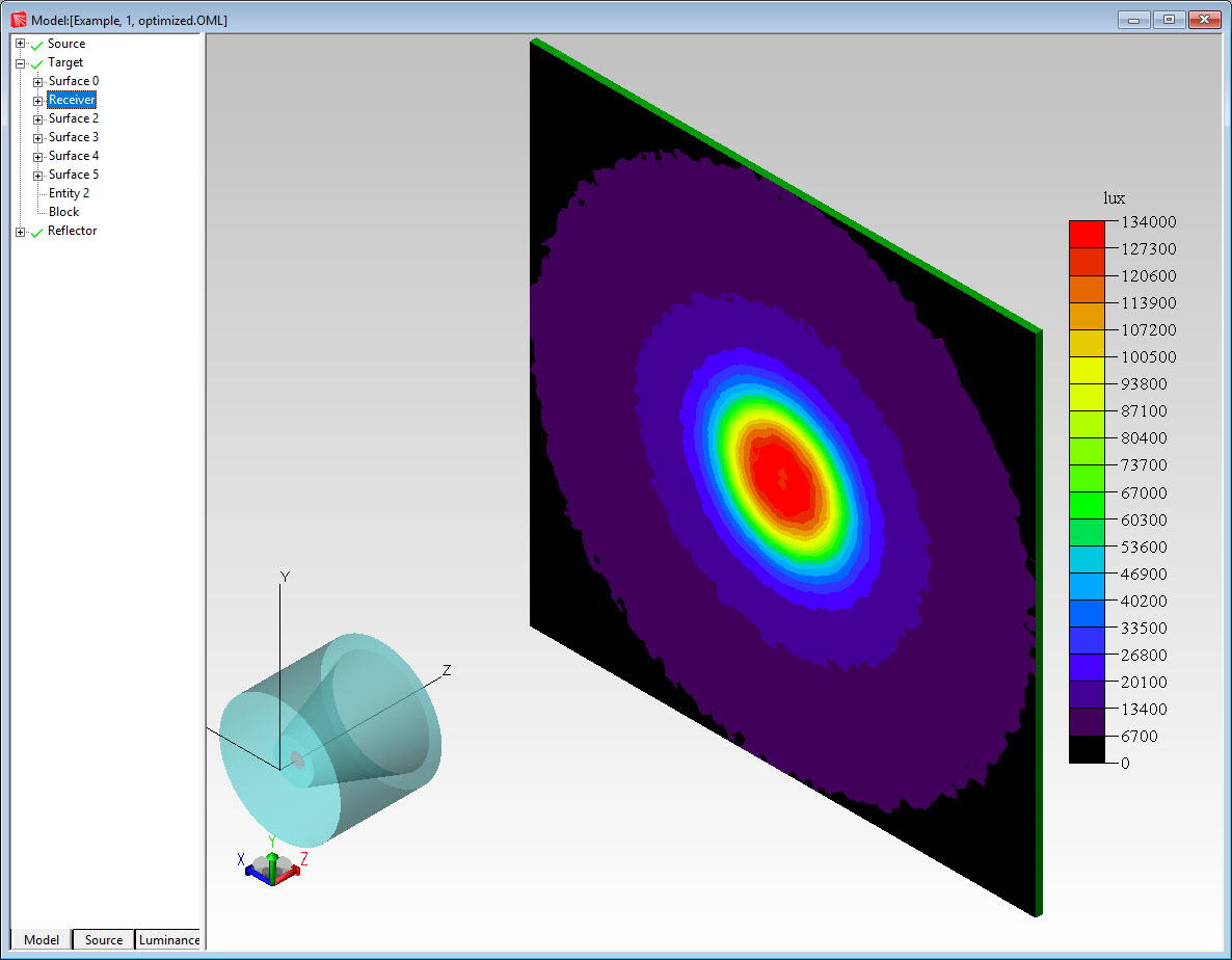
Figure 2: Optimized reflector and illumination pattern
In this example the end point of the reflector curve will be allowed to move. This variation could be the result of spring back or movement of the end of the reflector after it is molded or spun. The range of motion for this point is +/1mm horizontally. Figure 3 shows the point that can move and the range of motion during the tolerance analysis.
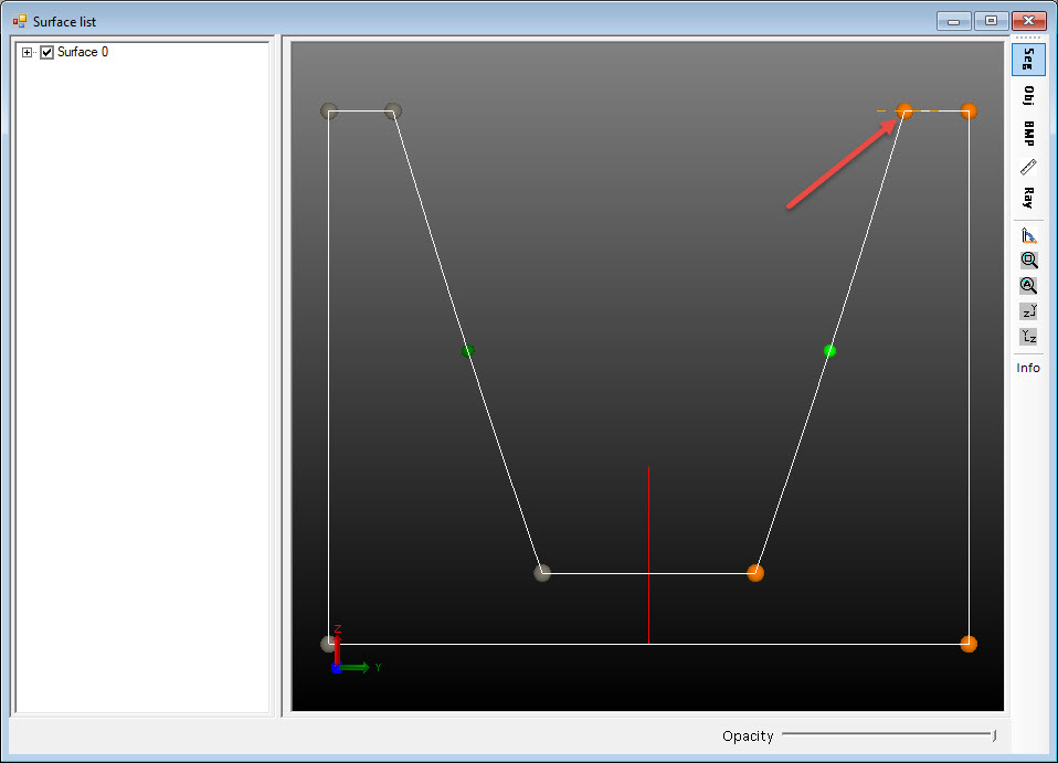 Figure 3: Reflector profile and point that can move +/- 1mm
The number of iterations for the tolerance analysis was set to 250 and the distribution method was Gaussian. Figure 4 shows the results of the tolerance analysis with the error along the X-axis and the accumulated ratio in percentage along the Y-axis. As can be seen, most of the results are on the left side of the plot with the lowest error function. This design should be fairly tolerant of changes due to manufacturing variations.

Figure 4: Accumulated error values for 250 iterations
Figure 5 shows the Error Value plotted as a function of the Variable Value. The variable value for the optimized condition was 7.178mm. The variable values for the best and worst-case conditions were 7.180mm and 6.180mm respectively. Figures 6 and 7 show the illumination pattern for the best and worst-case conditions respectively.
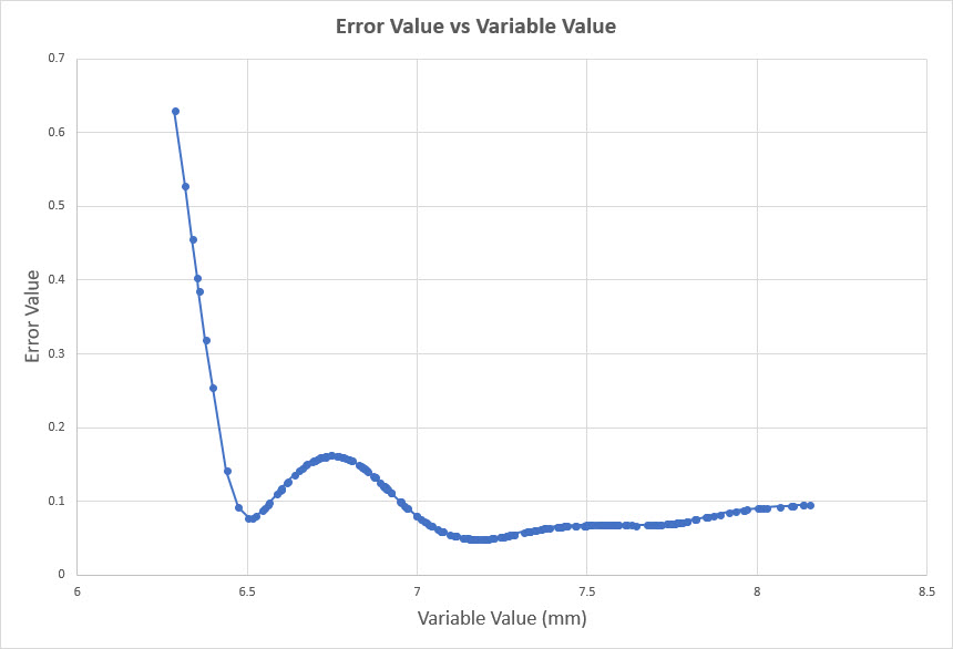
Figure 5: Error Value vs Variable Value
 Figure 6: Best-case illumination pattern
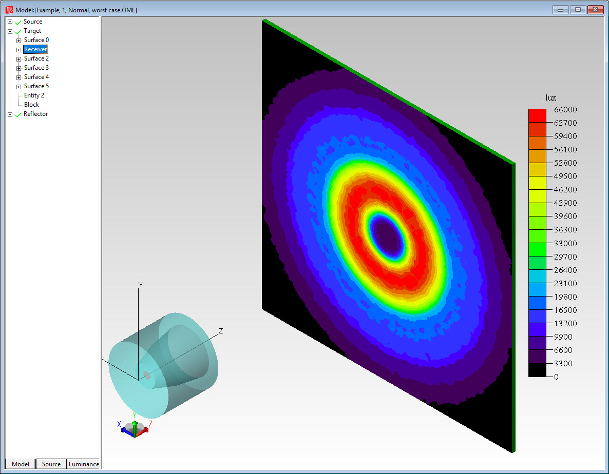 Figure 7: Worst-case illumination pattern
Example 2: CPC concentrator tolerance example
This example will show the tolerance analysis of a CPC (compound parabolic concentrator) reflector. The CPC is concentrating light onto a detector. Figure 8 shows the system layout.
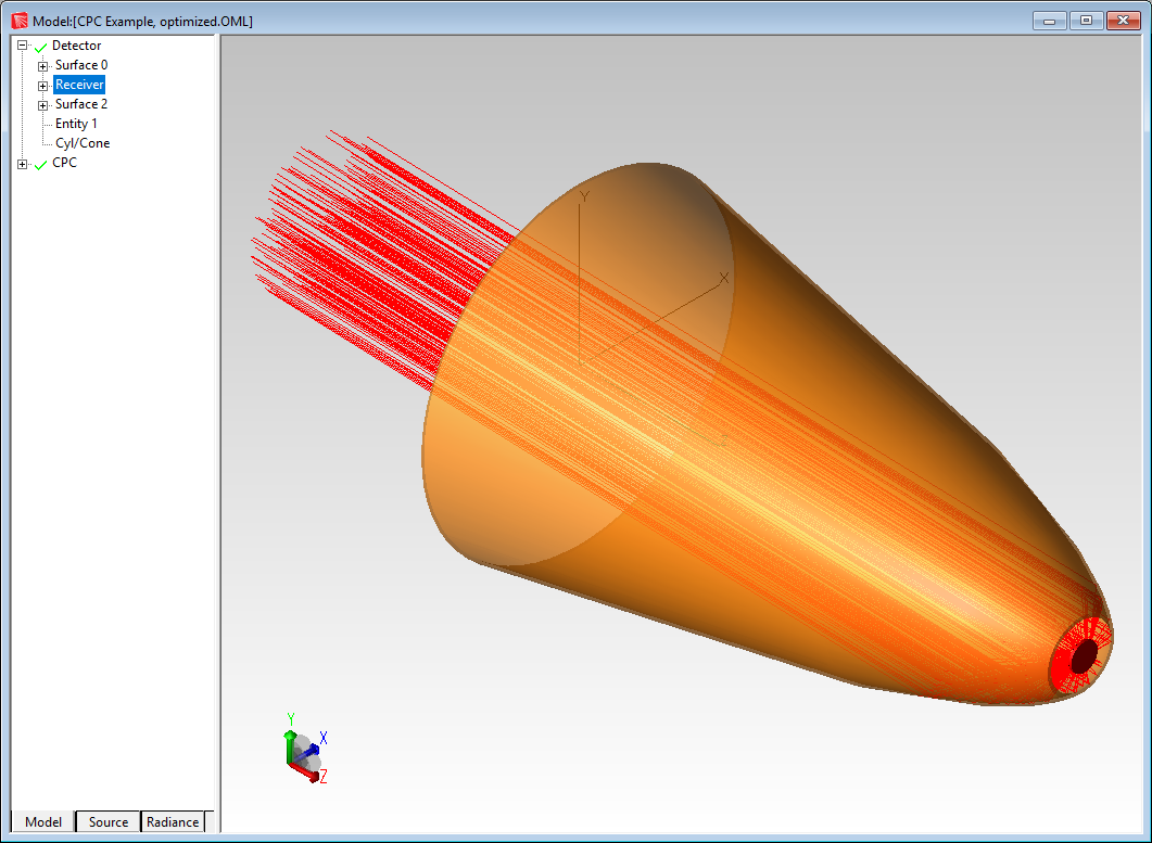 Figure 8: CPC concentrator
In this example the lateral focus shift and axis tile of the CPC was allowed to vary. The lateral focus shift was allowed to change +/- 1mm and the axis tilt was allowed to change +/- 1 degrees.
The number of iterations for the tolerance analysis was set to 500 and the distribution method was Gaussian, as in the previous example. The metric in this analysis was the peak irradiance on the detector. Figure 9 shows the results of the tolerance analysis with the error along the X-axis and the accumulated ratio in percentage along the Y-axis. Note that most of the results are on the left side of the plot which would initially suggest a tolerant design, but looking at the values of the error value they range from 142 to 6.657 x 10⁵. In this case the design is not very tolerant of changes to the optimized values.
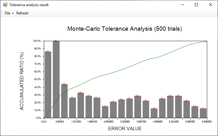
Figure 9: Accumulated error values for 500 iterations
Figures 10 and 11 show the irradiance pattern for the best and worst-case conditions respectively. The ration of the irradiance values is 4.15:1. The difference in the lateral shift and tilt angle between the optimal position and the worst case was about 1.5mm and 0.22-degrees respectively.
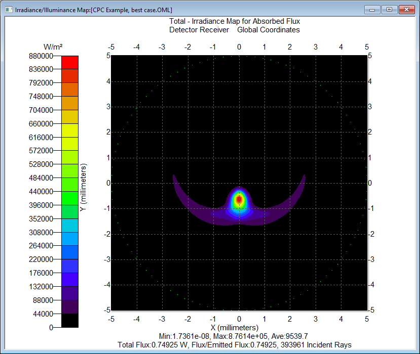 Figure 10: Best case irradiance pattern
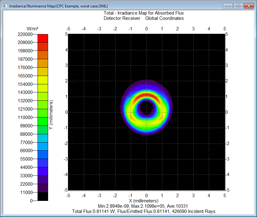
Figure 11: Worst case irradiance pattern
Conclusion
The ability to automate the tolerancing process has long been a feature of lens and imaging system design software but recently this capability has become available for illumination and non-imaging optical design and analysis programs. This ability gives the user the capability to test a design to see if it will perform as intended despite inevitable variations in the manufacturing process. Designs with a large variation in results can be improved or changed to make the resulting product more immune to process and manufacturing variations, improving the potential yield and reducing waste.
References
[1]OSLO Program Reference, Lambda Research Corporation